In this post I will be guiding you through the process of creating a simple spectral clustering algorithm. Spectral clustering allows us to find similarities in data points. In this simple tutorial, we will understand how to partition data into their natural clusters.

Motivation

First, let’s import the necessary libraries.

import numpy as np
from sklearn import datasets
from matplotlib import pyplot as plt

To motivate spectral clustering, we must understand when we can use it, and when we do not need to. Here is an example of a set of points.

n = 200
np.random.seed(1111)
X, y = datasets.make_blobs(n_samples=n, shuffle=True, random_state=None, centers = 2, cluster_std = 2.0)
plt.scatter(X[:,0], X[:,1])

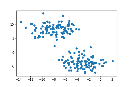
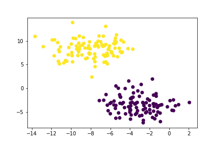
Here we can see two natural “blobs” of points. K-means clustering groups points from their average distance to the center of each circular cluster. We can see that K-means is very effective in separating the two blobs and thus spectral clustering is not needed.

from sklearn.cluster import KMeans
km = KMeans(n_clusters = 2)
km.fit(X)

plt.scatter(X[:,0], X[:,1], c = km.predict(X))

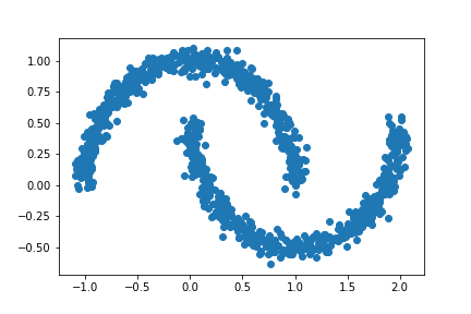
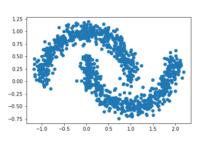
Now here is another example of data points in two intuitive clusters.

np.random.seed(1234)
n = 200
X, y = datasets.make_moons(n_samples=n, shuffle=True, noise=0.05, random_state=None)
plt.scatter(X[:,0], X[:,1])

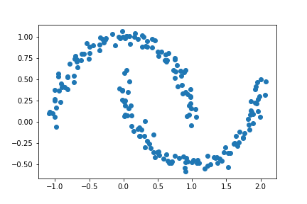
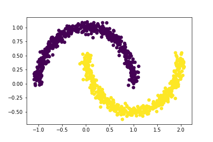
Below, we can see that K-means is not as effective at differentiating the two crescents.

km = KMeans(n_clusters = 2)
km.fit(X)
plt.scatter(X[:,0], X[:,1], c = km.predict(X))

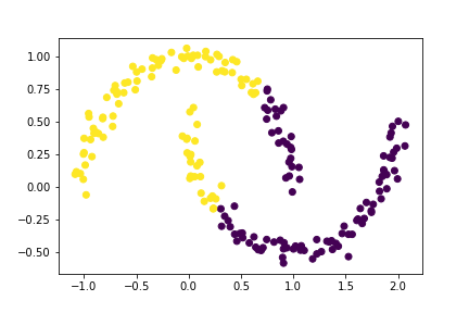
Using spectral clustering we will be able to correctly identify the two crescents.

Part A: The Similarity Matrix

We will begin by creating the similarity matrix A. Given n data points, A is a nxn matrix of 0s and 1s and is reliant on a parameter epsilon. The ith, jth entry of A is 1 if the distance between the ith and jth data points are within epsilon of each other. Thus an entry of 0 would indicate that the ith and jth data points are greater than epsilon apart. Furthermore, the diagonal entries will all be 0.

We will use the function euclidean_distances from sklearn here. This function computes the distances between the all the points and returns them in a matrix. Then we compare these distances to epsilon to create the similarity matrix.

from sklearn.metrics.pairwise import euclidean_distances
epsilon = 0.4
A = euclidean_distances(X, X) # computes distances between ith and jth points
A[A < epsilon] = 1 # points within epsilon distance are 1
A[A != 1] = 0 # other points are 0
np.fill_diagonal(A, 0) # set diagonal entries equal to 0
A

array([[0., 0., 0., ..., 0., 0., 0.],
       [0., 0., 0., ..., 0., 0., 0.],
       [0., 0., 0., ..., 0., 1., 0.],
       ...,
       [0., 0., 0., ..., 0., 1., 1.],
       [0., 0., 1., ..., 1., 0., 1.],
       [0., 0., 0., ..., 1., 1., 0.]])

We can see that the output is an array of 0s and 1s with 0s on the diagonal. As a sanity check, let’s see if A is symmetric.

np.all(A.T==A) # check that A is symmetric

True

We can see that the similarity matrix is symmetric. This means A[i, j] equals A[j, i] for all i, j. This is expected because the distance between the ith and jth points is equal to the distance between the jth and ith points.

Part B: The Binary Norm Cut Objective

The binary norm cut objective of a matrix A is the function

This is an intense formula but we will break it down.

• \(C_0\) and \(C_1\) represent the two clusters of data points.
• cut term: \(\mathbf{cut}(C_0, C_1) \equiv \sum_{i \in C_0, j \in C_1} a_{ij}\)
• volume term: \(\mathbf{vol}(C_0) \equiv \sum_{i \in C_0}d_i\), where \(d_i = \sum_{j = 1}^n a_{ij}\)

We want to minimize \(N_{\mathbf{A}}(C_0, C_1)\) because this will indicate that the clustering is a good partition of the points.

The Cut Term

Recall the \(C_0\) and \(C_1\) represent the two clusters of points. The cut term is the number points in different clusters (one in \(C_0\) and the other in \(C_1\)) that are within a distance epsilon of each other. This means that the corresponding entry in A will be 1. We want the cut term to be small because we don’t want points in \(C_0\) to be close to points in \(C_1\). We calculate the cut by summing the entries A[i, j] where i and j are in different clusters.

def cut(A, y):
    cut = 0
    for i in range(len(y)):
        for j in range(len(y)):
            if y[i] != y[j]: # points in different clusters
                cut += A[i,j] # add to cut term
    return cut

Let’s compute the cut term for the true clusters. Recall, A is the similarity matrix we constructed, and y is a binary vector that contains the actual labels of which cluster each point is in.

print(cut(A, y))

26.0

Without any scale, it is hard to know whether 26 is a large or small cut size. Let’s create a random binary vector to replace y and see what the cut term is.

rand = np.random.randint(2, size = 200) # random vector with 200 entries of 0s or 1s
print(cut(A, rand))

2300.0

As we can see, our cut term for the data is significantly smaller than the cut term when the points are randomly labelled.

The Volume Term

The volume of a cluster measures how large the cluster is. In the binary norm cut objective equation, the volume terms are in the denominator. Since we want \(\frac{1}{\mathbf{vol}(C_0)} + \frac{1}{\mathbf{vol}(C_1)}\) to be small, we don’t want \(C_0\) or \(C_1\) to be too small. Below is the function that returns the volume of each cluster as a tuple.

def vols(A, y):
    return (sum(sum(A)[y == 0]), sum(sum(A)[y == 1]))

Creating the Binary Normalized Cut Objective

Now that we have created functions for the cut and volume terms, we can but these together to calculate the binary normalized cut objective of matrix A with clustering vector y.

def normcut(A, y):
    v0, v1 = vols(A, y)
    return cut(A, y) * ((1 / v0) + (1 / v1))

To check if our function is working properly, we will compare the binary normalized cut objective of A using the real cluster labels y and the randomly generated labels rand from above.

print(normcut(A, y))
print(normcut(A, rand))

0.02303682466323045
2.0480047195518316

As we can see, the correct binary normalized cut objective is almost 100 times smaller than the randomly created one. This confirms that our binary normalized cut objective is small, as desired.

Part C: A Math Trick

We just found a way to calculate the binary normalized cut objective of A, however this is computationally intensive. When calculating the cut term, we used a nested for loop, and this is very slow. Instead here is another way to define the binary normalized cut objective.

Let z be a new vector such that:

D is a diagonal matrix with nonzero entries \(d_{ii} = d_i\), and where \(d_i = \sum_{j = 1}^n a_i\) is the degree (row-sum) from before.

We can rewrite the binary normalized cut objective as:

Let’s create a function that can compute the z vector.

def transform(A, y):
    z = np.zeros(n) # set z to have n elements
    v0, v1 = vols(A, y)

    # set elements of z based on cluster
    z[y == 0] = 1 / v0
    z[y == 1] = -1 / v1
    return z

Now, let’s check if the new binary normalized cut objective is equal to the one we calculated in part B.

z = transform(A, y)
D = np.diag(sum(A))
check = 2 * (np.transpose(z)@(D-A)@z) / (z@D@z) # new formula
print(check, normcut(A, y))
print(np.isclose(check, normcut(A, y)))

0.02303682466323018 0.02303682466323045
True

We can see that the new formula for the binary normalized cut objective produces a value extremely close to the original one we calculated. In fact, the difference is so small that it is less than the error that the computer has in calculating them.

Let’s also check if \(\mathbf{z}^T\mathbf{D}\mathbb{1} = 0\). This will check if z is constructed correctly.

print(np.transpose(z)@D@np.ones(200))
print(np.isclose(np.transpose(z)@D@np.ones(200), 0))

-2.7755575615628914e-17
True

As we can see, \(\mathbf{z}^T\mathbf{D}\mathbb{1}\) is an extremely small value. The difference between it and 0 is less than the error a computer has in calculating it. Thus we have verified the identity and z has been constructed correctly.

Part D: Minimizing the Function

We have just found a new formula for the binary normalized cut objective. We will label this \(R_A(z)\) for clarity.

Thus, minimizing the binary normalized cut objective is equivalent to minimizing \(R_A(z)\). We will minimize \(R_A(z)\) by minimizing the difference between z and its orthogonal component.

def orth(u, v):
    return (u @ v) / (v @ v)*v

e = np.ones(n)

d = D @ e

def orth_obj(z):
    z_o = z - orth(z, d)
    return (z_o @ (D - A) @ z_o)/(z_o @ D @ z_o)

from scipy.optimize import minimize
z_ = minimize(orth_obj, z).x

Now, z_ is a vector that contains the value of z that minimizes \(R_A(z)\).

Part E: Checking Our Work So Far

Recall, z is designed such that the sign of z indicates which cluster it is in. Let’s check and see if the sign of our minimized z_ will separate the two clusters. Due to the nature of this optimization problem, the actual cutoff is -0.0015 rather than 0.

bnd = -0.0015
plt.scatter(X[:,0][z_ < bnd], X[:,1][z_ < bnd], c = 'purple')
plt.scatter(X[:,0][z_ >= bnd], X[:,1][z_ >= bnd], c = 'yellow')

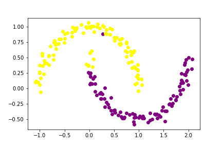
Wow! For the most part, it looks like our data has been clustered correctly.

Part F: A Linear Algebra Solution

The optimization we did in part D was effective, however it was very slow. Instead we will use the Laplacian matrix L and find its second smallest eigenvalue and corresponding eigenvector. This eigenvector will be our new z vector that labels the clusters.

L = np.linalg.inv(D)@(D-A) # create the Laplacian matrix
eig_vals, eig_vecs = np.linalg.eig(L) # compute eigenvalues and eigenvectors of Laplacian matrix
idx = np.argsort(eig_vals) # find indexes eigenvalues sorted in ascending order
eig_vals, eig_vecs = eig_vals[idx], eig_vecs[:,idx] # sort eigenvalues and eigenvectors by ascending order of eigenvalues
z_eig = eig_vecs[:,1] # obtain eigenvector corresponding to second smallest eigenvalue

z_eig = np.linalg.eig(L)[1][:,1]

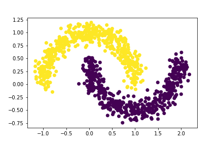
# color the points based on the sign of z_eig
plt.scatter(X[:,0][z_eig  < 0], X[:,1][z_eig  < 0], c = 'purple')
plt.scatter(X[:,0][z_eig  >= 0], X[:,1][z_eig  >= 0], c = 'yellow')

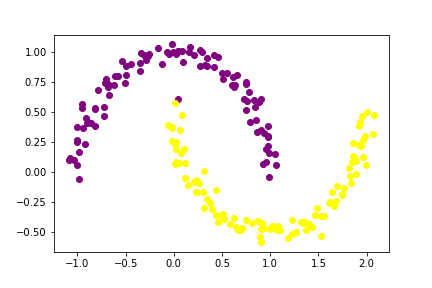
And again we have the crescents clustered! The linear algebra solution is more efficient than the explicit optimization from part D. This is where the name spectral clustering comes from since it uses the eigenvalues and eigenvectors of A.

Part G: Putting it all together

Now we have explored how to use spectral clustering to separate the two crescents. Let’s put everything we have learned into a function!

def spectral_clustering(X, epsilon):
    """
    Arguments:
    X: an array of points with x and y coordinates
    epsilon: a small value which defines the cutoff for points being close together

    Returns:
    A binary vector labelling which cluster each respective point belongs to
    """

    # Construct the similarity matrix A
    A = euclidean_distances(X, X)
    A[A < epsilon] = 1
    A[A != 1] = 0
    np.fill_diagonal(A, 0)

    # Construct the Laplacian matrix
    D = np.diag(sum(A))
    L = np.linalg.inv(D)@(D-A)

    # Compute eigenvector with second smallest eigenvalue of L
    eig_vals, eig_vecs = np.linalg.eig(L)
    idx = np.argsort(eig_vals)
    eig_vals, eig_vecs = eig_vals[idx], eig_vecs[:,idx]
    z_eig = eig_vecs[:,1]

    # Return labels based on eigenvector
    return 1 * (z_eig > 0)  

Part H: Experimenting with Crescents

Let’s test out our new function on different data sets.

Here is an example with more data points

np.random.seed(1000)
n = 1000
X, y = datasets.make_moons(n_samples=n, shuffle=True, noise=0.05, random_state=None)
plt.scatter(X[:,0], X[:,1])

Let’s try out our new spectral clustering function and see if it can separate the crescents.

test1 = spectral_clustering(X, 0.4)
plt.scatter(X[:,0], X[:,1], c = test1)

Our spectral clustering function was able to separate the two clusters!

plt.scatter(X[:,0][test1 == 1], X[:,1][test1 == 1], c = 'purple')
plt.scatter(X[:,0][test1 == 0], X[:,1][test1 == 0], c = 'yellow')

plt.scatter(X[:,0], X[:,1], c = test1)

Here’s an example with more noise.

n = 1000
X, y = datasets.make_moons(n_samples=n, shuffle=True, noise=0.1, random_state=None)
plt.scatter(X[:,0], X[:,1])

To compensate for the extra noise, I decreased the epsilon value.

test2 = spectral_clustering(X, 0.3)
plt.scatter(X[:,0], X[:,1], c = test2)

As you can see, our spectral clustering function is able to separate the two crescents!

Part I: Bull’s Eye

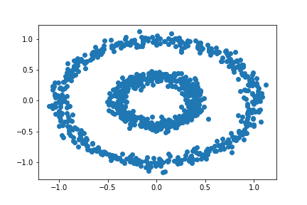
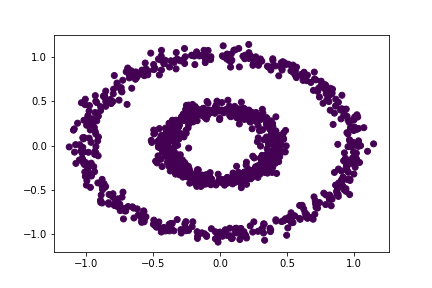
What if we have a different data set? Let’s try a bull’s eye.

n = 1000
X, y = datasets.make_circles(n_samples=n, shuffle=True, noise=0.05, random_state=None, factor = 0.4)
plt.scatter(X[:,0], X[:,1])

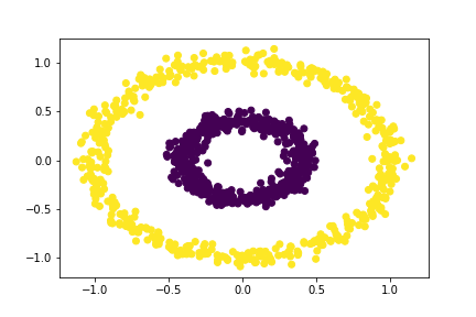
Will k-means clustering work?

km = KMeans(n_clusters = 2)
km.fit(X)
plt.scatter(X[:,0], X[:,1], c = km.predict(X))

Again, k-means clustering is not effective here.

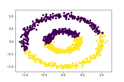
Let’s try our spectral clustering function!

bull = spectral_clustering(X, 0.3)
plt.scatter(X[:,0], X[:,1], c = bull)

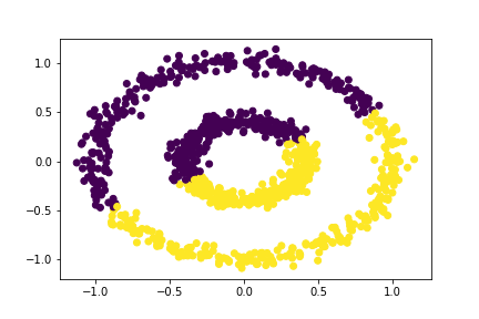
Hmmm this didn’t seem to work. Let’s try increasing the value of epsilon to 0.4.

bull = spectral_clustering(X, 0.4)
plt.scatter(X[:,0], X[:,1], c = bull)

Great! Our spectral clustering function was able to separate the two concentric circles. Let’s see what other values of epsilon can separate the circles.

bull = spectral_clustering(X, 0.5)
plt.scatter(X[:,0], X[:,1], c = bull)

An epsilon value of 0.5 also separates the circles!

bull = spectral_clustering(X, 0.6)
plt.scatter(X[:,0], X[:,1], c = bull)

Look’s like an epsilon value of 0.6 is not able to separate the circles. Thus, epsilon values between 0.4 and 0.5 can distinguish the two circles.

Thanks for reading my post about spectral clustering. I hope you learned something new today!