
Identifying Fake News with TensorFlow
In this post, I’ll explain how to create a fake news classifier using TensorFlow. We will be creating three models to predict whether news articles contain fake news, and then evaluate them.
There are quite a few steps, so here is the process we will follow.
- Acquire Training Data
- Create a Dataset
- Preprocessing
- Creating the Title Model
- Creating the Text Model
- Creating the Combined Model
- Testing Out the Model
- Visualizing
Before we get into it, let’s download the necessary packages. As we can see, we will need many functionalities of TensorFlow.
import tensorflow as tf
from tensorflow.keras.layers.experimental.preprocessing import TextVectorization
from tensorflow import keras
from tensorflow.keras import layers
from tensorflow.keras import losses

import pandas as pd
import re
import string
from matplotlib import pyplot as plt
import numpy as np
import plotly.express as px

import nltk
nltk.download('stopwords')
from nltk.corpus import stopwords
1. Acquire Training Data
The data that we will use to train the model can be found at the link below.
train_url = "https://github.com/PhilChodrow/PIC16b/blob/master/datasets/fake_news_train.csv?raw=true"
Let’s read this data into a pandas dataframe.
train_data = pd.read_csv(train_url)
train_data
| Unnamed: 0 | title | text | fake | |
|---|---|---|---|---|
| 0 | 17366 | Merkel: Strong result for Austria's FPO 'big c... | German Chancellor Angela Merkel said on Monday... | 0 |
| 1 | 5634 | Trump says Pence will lead voter fraud panel | WEST PALM BEACH, Fla.President Donald Trump sa... | 0 |
| 2 | 17487 | JUST IN: SUSPECTED LEAKER and “Close Confidant... | On December 5, 2017, Circa s Sara Carter warne... | 1 |
| 3 | 12217 | Thyssenkrupp has offered help to Argentina ove... | Germany s Thyssenkrupp, has offered assistance... | 0 |
| 4 | 5535 | Trump say appeals court decision on travel ban... | President Donald Trump on Thursday called the ... | 0 |
| ... | ... | ... | ... | ... |
| 22444 | 10709 | ALARMING: NSA Refuses to Release Clinton-Lynch... | If Clinton and Lynch just talked about grandki... | 1 |
| 22445 | 8731 | Can Pence's vow not to sling mud survive a Tru... | () - In 1990, during a close and bitter congre... | 0 |
| 22446 | 4733 | Watch Trump Campaign Try To Spin Their Way Ou... | A new ad by the Hillary Clinton SuperPac Prior... | 1 |
| 22447 | 3993 | Trump celebrates first 100 days as president, ... | HARRISBURG, Pa.U.S. President Donald Trump hit... | 0 |
| 22448 | 12896 | TRUMP SUPPORTERS REACT TO DEBATE: “Clinton New... | MELBOURNE, FL is a town with a population of 7... | 1 |
22449 rows × 4 columns
We see that this dataset contains information about 22449 articles. Each row represents an article and there are three columns that contain the title, the full article text, and a boolean value that indicates whether the article is fake or not. This fake column is 0 when the article is true and 1 when the article contains fake news.
2. Create a Dataset
We’re going to create a function called make_dataset. This will convert our pandas dataframe to a TensorFlow Dataset. This allows us to stay organized while creating our data pipeline. In this function, we will remove stop words from the title and text columns of each article. Stop words in English are words like “the”, “and”, or “but”. We use a lambda function which loops through all the words, and then removes the word if it is a stopword as determined in the nltk package.
A peer suggested that I add more explanation regarding the make_dataset function because contains many trick steps such as getting the stopwords from nltk and using lambda functions.
Then we will define the input and output components of our dataset. We want the model to evaluate the title and text of the article, so these are the inputs. The output will be 0 or 1, depending if the article contains fake news or not.
def make_dataset(train_data):
  # get list of stopwords from nltk
  stop = stopwords.words('english')

  # remove stopwords from titles
  train_data['title'] = train_data['title'].apply(lambda x: ' '.join([word for word in x.split() if word not in (stop)]))

  # remove stopwords from text
  train_data['text'] = train_data['text'].apply(lambda x: ' '.join([word for word in x.split() if word not in (stop)]))

  # create TensorFlow dataset
  data = tf.data.Dataset.from_tensor_slices(
    (
        {
            "title" : train_data[["title"]],
            "text" : train_data[["text"]]
        },
        {
            "fake" : train_data[["fake"]]
        }
    )
)
  data.batch(100) # batching the data allows it to efficiently train in chunks

  return data
Let’s use our make_dataset function on our pandas dataframe.
data = make_dataset(train_data)
Now let’s split our data into training and validation sets. We will use 80% for training and 20% for validation. Again, we will batch the data so it will train more efficiently.
data = data.shuffle(buffer_size = len(data))

train_size = int(0.8 * len(data)) # allocate 80% of data for training

train = data.take(train_size).batch(100) # set training data
val = data.skip(train_size).batch(100) # set validation data
We can check to see the size of the sets train and val.
len(train), len(val)
(180, 45)
Here we see that the training data is four times larger than the validation data, which is what we expect. Because we batched the data, each value here actually represents 100 articles. Thus this sums to 22500 articles, which is roughly the amount of articles in our original pandas dataframe.
3. Preprocessing
Before we get into the models, we need to do some data cleaning. The first step is to standardize the data. We will accomplish this by turning all the text to lower case and then removing any punctuation. This is where we use the re (regular expression) and string libraries.
def standardization(input_data):
    lowercase = tf.strings.lower(input_data) # all letters to lowercase
    no_punctuation = tf.strings.regex_replace(lowercase,
                                  '[%s]' % re.escape(string.punctuation),'') # remove punctuation
    return no_punctuation
Next, we will vectorize the data. In this case, we will convert our text data into numbers so that our models will be able to understand them. The number associated with each word represents how frequently it appears in the dataset. This means a word with a vectorized value of 347 is the 347th most popular word in the data. I have arbitrarily decided to only consider the top 5000 words in the dataset.
size_vocabulary = 5000

vectorize_layer = TextVectorization(
    standardize=standardization,
    max_tokens=size_vocabulary, # only consider this many words
    output_mode='int',
    output_sequence_length=500)
Let’s apply the vectorization to the title and text columns of the dataset! Here lambda functions are used to apply the vectorization to all the titles and texts of the articles.
vectorize_layer.adapt(train.map(lambda x, y: x["title"]))
vectorize_layer.adapt(train.map(lambda x, y: x["text"]))
As a last step before creating the models, we will define the input types of the data. The inputs title and text are both one dimensional vectors of strings, and this is reflected in the following code.
title_input = keras.Input(
    shape = (1,),
    name = "title",
    dtype = "string"
)

text_input = keras.Input(
    shape = (1,),
    name = "text",
    dtype = "string"
)
4. Creating the Title Model
The first model we will create will determine whether an article contains fake news or not solely based on its title. To do so, we will use the functional API of TensorFlow. We will define a pipeline of hidden layers to process the titles. First, we explicitly define an embedding layer. This is so we can reuse it in a later model. Then we define different layers for the text data. The dropout layers prevent overfitting.
embedding = layers.Embedding(size_vocabulary, 12, name = "embedding") # define an embedding layer

title_features = vectorize_layer(title_input) # vectorize the title inputs
title_features = embedding(title_features) # use the defined embedding layer
title_features = layers.Dropout(0.2)(title_features) # prevent overfitting
title_features = layers.GlobalAveragePooling1D()(title_features)
title_features = layers.Dropout(0.2)(title_features) # prevent overfitting
title_features = layers.Dense(32, activation='relu')(title_features)
I gave a suggestion to a classmate to create an embedding layer independent of the models. This allows all the models to share the embedding layer and then one single text embedding visualization can be created from it.
Now we will add an additional dense layer and then define the output. Recall, we want the output to be 0 or 1 depending on whether the article contains fake news. Since there are only 2 options for the output, the number of units of the layer is 2, and notice we name it fake.
main_title = title_features
main_title = layers.Dense(32, activation='relu')(main_title)
output_title = layers.Dense(2, name = "fake")(main_title)
Now let’s put the model together by defining the inputs and outputs.
model_title = keras.Model(
    inputs = title_input,
    outputs = output_title
)
Let’s look at a diagram that represents the layers of the model to understand its structure.
keras.utils.plot_model(model_title)
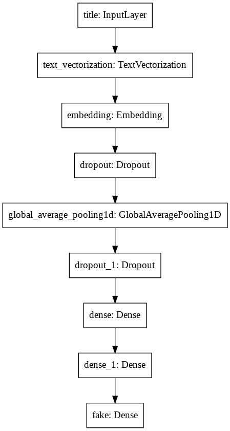
We can see how the title is vectorized, passed through the embedding layer, and then continues through multiple layers until the end when it outputs fake.
Let’s compile model_title.
model_title.compile(optimizer = "adam",
              loss = losses.SparseCategoricalCrossentropy(from_logits=True),
              metrics=['accuracy']
)
Now we can run model_title. Notice we use the training and the validation data. The number of epochs represents how many times the model is trained.
history_title = model_title.fit(train,
                    validation_data=val,
                    epochs = 20)
Epoch 1/20
/usr/local/lib/python3.7/dist-packages/tensorflow/python/keras/engine/functional.py:595: UserWarning: Input dict contained keys ['text'] which did not match any model input. They will be ignored by the model.
  [n for n in tensors.keys() if n not in ref_input_names])
180/180 [==============================] - 5s 21ms/step - loss: 0.6925 - accuracy: 0.5135 - val_loss: 0.6870 - val_accuracy: 0.5276
Epoch 2/20
180/180 [==============================] - 3s 16ms/step - loss: 0.6411 - accuracy: 0.6493 - val_loss: 0.2182 - val_accuracy: 0.9508
Epoch 3/20
180/180 [==============================] - 3s 16ms/step - loss: 0.1736 - accuracy: 0.9507 - val_loss: 0.1064 - val_accuracy: 0.9615
.....
Epoch 18/20
180/180 [==============================] - 3s 16ms/step - loss: 0.0259 - accuracy: 0.9915 - val_loss: 0.0187 - val_accuracy: 0.9947
Epoch 19/20
180/180 [==============================] - 3s 17ms/step - loss: 0.0245 - accuracy: 0.9921 - val_loss: 0.0205 - val_accuracy: 0.9947
Epoch 20/20
180/180 [==============================] - 3s 16ms/step - loss: 0.0238 - accuracy: 0.9922 - val_loss: 0.0163 - val_accuracy: 0.9947
Initially, I printed the output from all 20 epochs, and it was quite overwhelming. A peer suggested that I condense these outputs, since the following graph shows more clearly how the accuracy of the model changes with each epoch.
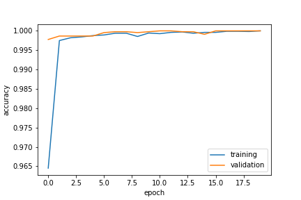
After 20 epochs, the model is has over 99% accuracy on both the training and validation data. This is great! Let’s visualize the accuracy over time.
plt.plot(history_title.history["accuracy"], label = "training")
plt.plot(history_title.history["val_accuracy"], label = "validation")
plt.gca().set(xlabel = "epoch", ylabel = "accuracy")
plt.legend()
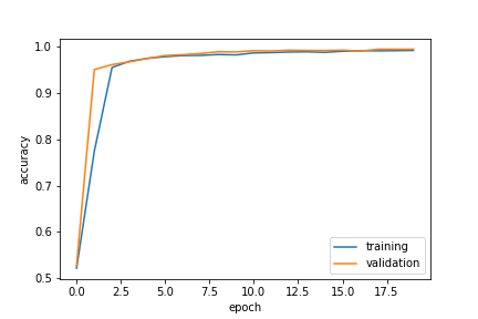
We can see that the training and validation data appear to have similar accuracy, which indicates we did not overfit the model. Additionally, the accuracies of both have “leveled off” so we probably would not benefit from more training. Our first model is complete!
I gave a suggestion to a classmate to plot the accuracy of the model. This makes it easier to see when the model is done training or whether it could benefit from additional training.
5. Creating the Text Model
For the second model, we will determine whether an article contains fake news or not solely based on the article text. This process will be very similar to the process above for creating the title model. We begin by creating some layers for the text input. Notice we use the embedding layer that we defined above.
text_features = vectorize_layer(text_input) # vectorize the text
text_features = embedding(text_features) # use defined embedding layer
text_features = layers.Dropout(0.2)(text_features) # prevent overfitting
text_features = layers.GlobalAveragePooling1D()(text_features)
text_features = layers.Dropout(0.2)(text_features) # prevent overfitting
text_features = layers.Dense(32, activation='relu')(text_features)
Again, we add another dense layer, and then create the output layer which only has 2 possible values. Then we put the model together by defining its inputs and outputs.
main_text = text_features
main_text = layers.Dense(32, activation='relu')(main_text)
output_text = layers.Dense(2, name = "fake")(main_text) # output layer

# create model
model_text = keras.Model(
    inputs = text_input,
    outputs = output_text
)
Let’s look at the diagram to better understand the structure of the model.
keras.utils.plot_model(model_text)
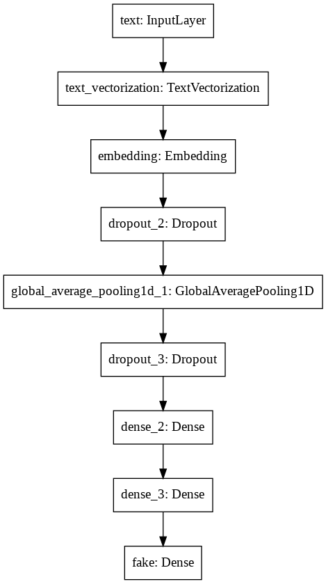
This diagram is very similar to the one for model_title since both have the same structure.
Now let’s compile our model and train it.
# compile the model
model_text.compile(optimizer = "adam",
              loss = losses.SparseCategoricalCrossentropy(from_logits=True),
              metrics=['accuracy']
)

# train the model
history_text = model_text.fit(train,
                    validation_data=val,
                    epochs = 20)
Epoch 1/20
/usr/local/lib/python3.7/dist-packages/tensorflow/python/keras/engine/functional.py:595: UserWarning: Input dict contained keys ['title'] which did not match any model input. They will be ignored by the model.
  [n for n in tensors.keys() if n not in ref_input_names])
180/180 [==============================] - 5s 26ms/step - loss: 0.5729 - accuracy: 0.7164 - val_loss: 0.2078 - val_accuracy: 0.9341
Epoch 2/20
180/180 [==============================] - 4s 24ms/step - loss: 0.1857 - accuracy: 0.9358 - val_loss: 0.1392 - val_accuracy: 0.9604
Epoch 3/20
180/180 [==============================] - 4s 25ms/step - loss: 0.1451 - accuracy: 0.9579 - val_loss: 0.1103 - val_accuracy: 0.9715
.....
Epoch 18/20
180/180 [==============================] - 5s 25ms/step - loss: 0.0124 - accuracy: 0.9969 - val_loss: 0.0078 - val_accuracy: 0.9987
Epoch 19/20
180/180 [==============================] - 5s 25ms/step - loss: 0.0128 - accuracy: 0.9969 - val_loss: 0.0077 - val_accuracy: 0.9987
Epoch 20/20
180/180 [==============================] - 5s 25ms/step - loss: 0.0152 - accuracy: 0.9954 - val_loss: 0.0104 - val_accuracy: 0.9976
Again, we can see that the model achieves over 99% accuracy on the training and validation data. Let’s plot its progress.
plt.plot(history_text.history["accuracy"], label = "training")
plt.plot(history_text.history["val_accuracy"], label = "validation")
plt.gca().set(xlabel = "epoch", ylabel = "accuracy")
plt.legend()
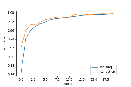
We can see that the validation data has a slightly higher accuracy than the training data, so we did not overfit the model. Both lines have “leveled off” so we are done training this model!
6. Creating the Combined Model
The last model will use both the title and text of the article to determine whether the article contains fake news. Since we have already defined the layers for title_features and text_features, we can combine them to create our new model.
main = layers.concatenate([title_features, text_features], axis = 1) # combine the layers of title and text
We will add another dense layer and then create our output layer. Then we can create the model by defining the inputs and outputs. Since we have two inputs this time, title_input and text_input are passed as a list.
main = layers.Dense(32, activation = 'relu')(main)
output = layers.Dense(2, name = "fake")(main)

model = keras.Model(
    inputs = [title_input, text_input],
    outputs = output
)
Let’s visualize the structure of the model.
keras.utils.plot_model(model)
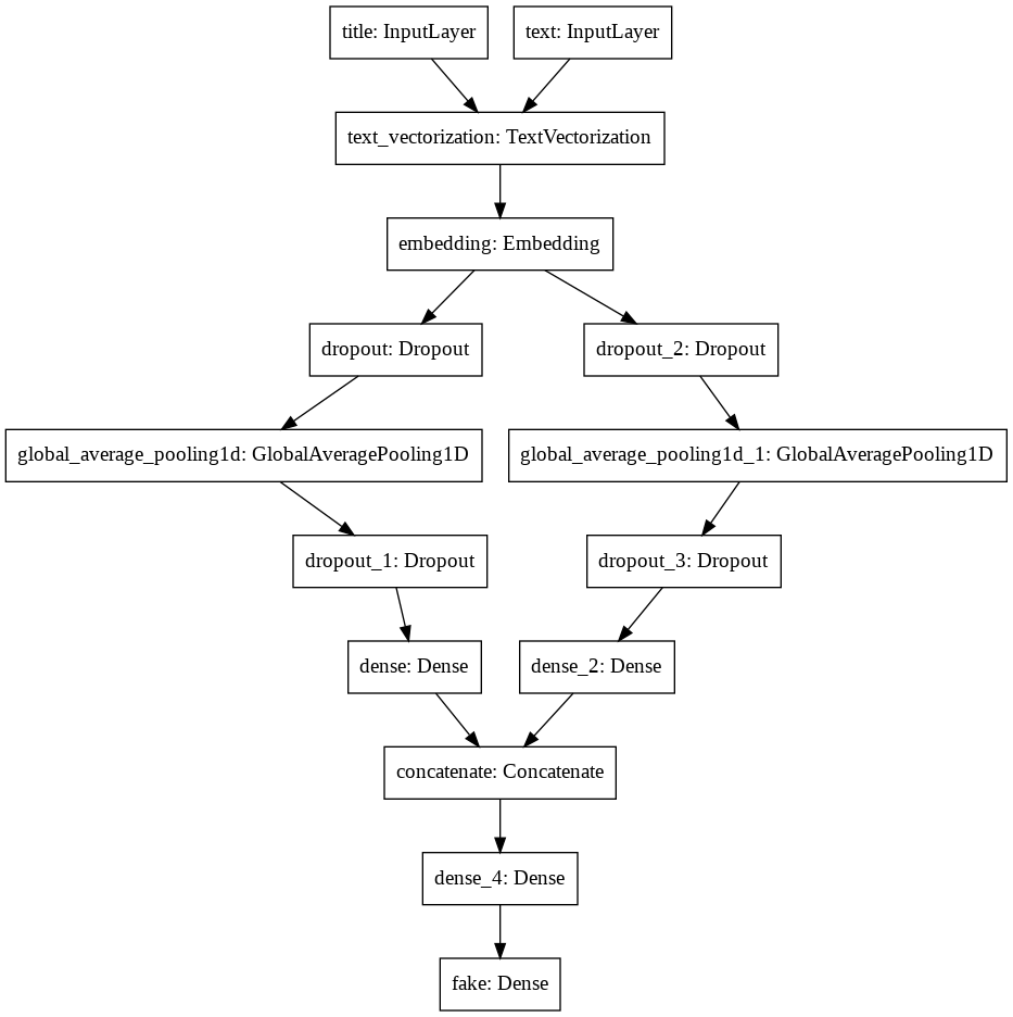
Notice how both the text and title go through the same embedding layer. Recall, we defined our own embedding layer and then had both the title and text use it. Another cool thing to note is how the two “branches” of layers come together at the concatenate layer. We explicitly did this when we created main. Let’s compile our model and train it.
# compile the model
model.compile(optimizer = "adam",
              loss = losses.SparseCategoricalCrossentropy(from_logits=True),
              metrics=['accuracy']
)

# train the model
history = model.fit(train,
                    validation_data=val,
                    epochs = 20)
Epoch 1/20
180/180 [==============================] - 8s 39ms/step - loss: 0.3635 - accuracy: 0.8894 - val_loss: 0.0369 - val_accuracy: 0.9978
Epoch 2/20
180/180 [==============================] - 7s 37ms/step - loss: 0.0299 - accuracy: 0.9975 - val_loss: 0.0136 - val_accuracy: 0.9987
Epoch 3/20
180/180 [==============================] - 7s 37ms/step - loss: 0.0148 - accuracy: 0.9978 - val_loss: 0.0099 - val_accuracy: 0.9987
.....
Epoch 18/20
180/180 [==============================] - 7s 38ms/step - loss: 6.7730e-04 - accuracy: 0.9998 - val_loss: 1.0663e-04 - val_accuracy: 1.0000
Epoch 19/20
180/180 [==============================] - 7s 37ms/step - loss: 2.7695e-04 - accuracy: 1.0000 - val_loss: 1.6648e-04 - val_accuracy: 1.0000
Epoch 20/20
180/180 [==============================] - 7s 37ms/step - loss: 5.2524e-04 - accuracy: 1.0000 - val_loss: 1.3989e-04 - val_accuracy: 1.0000
Wow! after 20 epochs we are able to get 100% accuracy on the training and validation data. Let’s visualize this.
plt.plot(history.history["accuracy"], label = "training")
plt.plot(history.history["val_accuracy"], label = "validation")
plt.gca().set(xlabel = "epoch", ylabel = "accuracy")
plt.legend()
We can see that the validation and training data reaches a similar level so we did not overfit the data. Additionally the accuracies have leveled off, so we are done training!
Since all three models are able to detect fake news in articles with at least 99% accuracy, I would recommend using the model with just title as it is the most efficient. However, if you are striving for the best accuracy, use the model with both title and text.
7. Testing Out the Model
Now, let’s test the model on data that it has never seen before. In this section I will use the model which has both title and text as inputs, but you could use any of the three models we created.
Let’s read in the test data. Like before, we will read the data into a pandas dataframe. Then we will use the make_dataset function that we created to convert it to a TensorFlow dataset.
test_url = "https://github.com/PhilChodrow/PIC16b/blob/master/datasets/fake_news_test.csv?raw=true"
test_data = pd.read_csv(test_url) # data to pandas dataframe
test = make_dataset(test_data) # convert data to Tensorflow dataset
Now we can use our model to evaluate the test data. We will batch the data for efficiency.
test_results = test.take(len(test)).batch(100)
model.evaluate(test_results)
225/225 [==============================] - 3s 14ms/step - loss: 0.0476 - accuracy: 0.9917
[0.047586873173713684, 0.9916700124740601]
Wow! We achieved 99% accuracy on the test data. Our model is great at detecting fake news in articles.
8. Visualizing
So our model can predict fake news with over 99% accuracy, but what has it learned? Let’s visualize this.
weights = model.get_layer('embedding').get_weights()[0] # get the weights from the embedding layer
vocab = vectorize_layer.get_vocabulary()                # get the vocabulary from our data prep for later

from sklearn.decomposition import PCA
pca = PCA(n_components=2)
weights = pca.fit_transform(weights)

embedding_df = pd.DataFrame({
    'word' : vocab,
    'x0'   : weights[:,0],
    'x1'   : weights[:,1]
})
Remember how we created an embedding layer? A word embedding allows us to visualize what the model learned about the words. Words that are similar should be close together while words that are different are far apart. We will use plotly to create an interactive plot so we can see how the words are related to each other. The words that the model associates with fake news will tend towards one side and the words that the model associates with real news will be on the other.
import plotly.express as px
fig = px.scatter(embedding_df,
                 x = "x0",
                 y = "x1",
                 size = list(np.ones(len(embedding_df))),
                 size_max = 2,
                 hover_name = "word")

fig.show()
On the far left we can see words such as “breaking”, “video”, and “watch” which remind me of clickbait. Other notable word on the left are “KKK”, “21wire” (a conspiracy new site), and “tucker” (maybe Tucker Carlson). It is clear that words on the left side are those that the model associates with fake news. On the right there are many country names such as “myanmar”, “russia”, and “chinas”. It seems that international news is less likely to be fake.
Thanks for reading this blog post about detecting fake news with TensorFlow. I hope you learned something new!